Higher Investment Best Way to Reduce Unemployment, Recent Experience Shows

 Some economists argue that the efforts now underway to reduce government spending as a share of GDP will have adverse effects on unemployment. This is not what the data show. Consider this chart which shows the pattern of government purchases as a share of GDP and the unemployment rate over the past two decades. (The data are quarterly seasonally adjusted from 1990Q1 to 2010Q3.) There is no indication that lower government purchases increase unemployment; in fact we see the opposite, and a time-series regression analysis to detect timing shows that the correlation is not due to any reverse causation from high unemployment to more government purchases.

graphscatgu

In sharp contrast, the data on spending shares show that the most effective way to reduce unemployment is to raise investment as a share of GDP. The second chart shows the relation between unemployment and fixed investment over the past two decades. Higher shares of investment are associated with lower unemployment.

graphscat

The time series in the third chart show the relationship from another perspective. Either way you look at it, the relationship between unemployment and the investment share is remarkably close. It holds for both non-residential and residential investment, and is a subject of my current research. Of the four shares of GDP (the other two of course being consumption and net exports), the investment share shows by far the largest negative association with unemployment.

graphtfiru

Encouraging the creation and expansion of businesses should be the focus on government efforts to reduce unemployment. The recent compromise agreement to prevent the increase in tax rates on small businesses and the move to lighten up on the anti-business sentiment coming out of Washington are two steps in the right direction.

Posted in Fiscal Policy and Reforms | Comments Off on Higher Investment Best Way to Reduce Unemployment, Recent Experience Shows

Higher Investment Best Way to Reduce Unemployment, Recent Experience Shows

Some economists argue that the efforts now underway to reduce government spending as a share of GDP will have adverse effects on unemployment. This is not what the data show. Consider this chart which shows the pattern of government purchases as a share of GDP and the unemployment rate over the past two decades. (The data are quarterly seasonally adjusted from 1990Q1 to 2010Q3.) There is no indication that lower government purchases increase unemployment; in fact we see the opposite, and a time-series regression analysis to detect timing shows that the correlation is not due to any reverse causation from high unemployment to more government purchases.In sharp contrast, the data on spending shares show that the most effective way to reduce unemployment is to raise investment as a share of GDP. The second chart shows the relation between unemployment and fixed investment over the past two decades. Higher shares of investment are associated with lower unemployment. The time series in the third chart show the relationship from another perspective. Either way you look at it, the relationship between unemployment and the investment share is remarkably close. It holds for both non-residential and residential investment, and is a subject of my current research. Of the four shares of GDP (the other two of course being consumption and net exports), the investment share shows by far the largest negative association with unemployment.
Encouraging the creation and expansion of businesses should be the focus on government efforts to reduce unemployment. The recent compromise agreement to prevent the increase in tax rates on small businesses and the move to lighten up on the anti-business sentiment coming out of Washington are two steps in the right direction.

Posted in Fiscal Policy and Reforms | Comments Off on Higher Investment Best Way to Reduce Unemployment, Recent Experience Shows

Historical Evidence on the Benefits of Rules-Based Economic Policies

Each year since 1948 the American Economic Association and the American Finance Association hold a joint luncheon with an invited speaker. Over the years the luncheon has grown to a very large affair usually held in the big hotel ballrooms. This year’s luncheon was held today in Denver, and I was the speaker. Like the first two speakers—Winthrop Aldrich, president of Chase National Bank, and Paul Douglas, U.S. Senator from Illinois and known to economists from the Cobb-Douglas production function—I spoke about monetary and fiscal policy. I presented evidence of an amazing six decade long correlation between rules-based policies and good economic performance. The correlation—along with basic economic reasoning—is strong evidence that rules-based monetary and fiscal policies are enormously beneficial to the economy. The historical swings away from rules toward discretion have been damaging whether during the Great Inflation of the 1970s or the recent Great Recession. Here is a copy of the speech and here is the video of the speech with introduction by AEA President elect Orley Ashenfelter (AEA ID is needed for video).

Posted in Teaching Economics | Comments Off on Historical Evidence on the Benefits of Rules-Based Economic Policies

New Revealing Study of FOMC References to the Fed’s Mandate

Dan Thornton of the Federal Reserve Bank of St. Louis just completed a very revealing paper called What Does the Change in the FOMC’s Statement of Objectives Mean? in which he traces FOMC references to the Fed’s mandate over many years. He documents a historically significant recent shift in the language with important legislative and policy implications. Until very recently the FOMC policy statement did not explicitly mention the “maximum employment” part of the dual mandate in the Federal Reserve Act. FOMC members preferred to refer to the goal of price stability and its role in creating strong economic and employment growth.

But on September 21, 2010 the FOMC changed the policy statement by starting to refer explicitly to “maximum employment.” It did so again following the November and the December FOMC meetings. The change coincides with efforts to promote QE2 and thereby provides factual evidence that the dual mandate was a factor in gaining support for this unconventional large-scale asset purchase program, an issue which has been debated recently as I wrote about here.

Dan Thornton also goes back further in time, documenting changes in the FOMC Directive. He finds no references to “maximum employment” from 1979, when Paul Volcker took over as Fed chair, until the language was inserted in the December 2008 Directive, just as the Fed was embarking on its first large scale asset purchases program, now called QE1.

Posted in Monetary Policy | Comments Off on New Revealing Study of FOMC References to the Fed’s Mandate

A Very Good Year for Economics Videos, Especially Cartoons

Short video clips are a good way to get students interested in economics and help them understand the basics. I especially like the Golden Balls video for teaching game theory and Milton Friedman’s classic telling of the pencil story for teaching price theory. The videos of Gerald Ford telling a joint session of Congress to “Whip Inflation Now”and of Arthur Burns telling a congressional committee that he would not increase the money supply are really good for macro.

2010 was a great year for new videos especially new cartoons, about which Amity Shlaes just posted a thoughtful article, Economics By Cartoon .

Here are some new videos which I think would be useful in the classroom if placed in context and used to generate discussion.

Quantitative Easing Explained. Already a classic, a friend first sent this to me by email on Nov 14, when it “only” had 100,000 downloads. It since went viral with 4 million downloads. Purists will note that it doesn’t get everything right, but the overall message is clear and correct; it will be good for generating class discussion, though it is particularly brutal in places. As Amity Shlaes points out, cartoon economics allows for a more basic “no holds barred” discussion with good “off the wall” questions, just the kind you want in an introductory economics class.

The Wrong Financial Adviser Created by my Stanford colleague and Nobel prize winner Bill Sharpe, this one uses the same cartoon making program used to create Quantitative Easing Explained, but, rather than taking on the Fed, it takes on financial advisers who charge too much and don’t deliver much value to investors. It has not gone viral yet, but it should because it satirically conveys important truths about investing. Combined with Burt Malkiel’s new little book Elements of Investing, with Charles Ellis, it will help students remember the lessons beyond the classroom when it really matters.

Bernanke on the Daily Show with Jon Stewart. This video includes a fascinating segment from two different episodes of 60 Minutes, in which the chairman gives two different answers about whether quantitative easing is printing money. Having students sort this one out will be a good “big think” exercise.

Unmasking Interest Rates, Honky Tonk Style. Produced by Paul Solman, this PBS video covers the monetary policy debate as of January 2010 and thus before QE2. It is pretty long for playing in class unless you edit or only play part. Here is a shorter version of the musical parts where (after a short intro by me) Merle Hazard sings “Inflation or Deflation”

Movie trailers can also prove useful if explained and put in context. The Inside Job Trailer and the Waiting for Superman Trailer are both very good as they address current events with deep economic significance. There is also a good clip of French Finance Minister Christine Lagarde from the movie Inside Job.

Finally I cannot forget to mention the very popular Hayek-Keynes rap “Fear the Boom and Bust” which came out in January 2010 and now has 1.7 million downloads.

Posted in Teaching Economics | Comments Off on A Very Good Year for Economics Videos, Especially Cartoons

Models Used for Policy Should Reflect Recent Experience, But Do They?

Data from the Department of Commerce show that short-term stimulus funds did not go to increase federal purchases, or state and local purchases, or even consumption purchases by much over the past few years. Thus the packages did not materially stimulate GDP or employment. In a recent Commentary piece “Where Did the Stimulus Go?” John Cogan and I review and explain our empirical research using these data.

Unfortunately, most Keynesian models have been not adjusted to incorporate these facts, so they keep making the same predictions. To cite one example, the multipliers in Mark Zandi’s model as of July 2008 are found here (page 52 of the full document, 5 of the paper) while the multipliers as of December 2010 are found here. They are virtually the same. The model assumes a multiplier from a temporary tax rebate or refund which is greater than one, even though the actual data show it was much less than one in the case of the 2008 and 2009 stimulus packages. Note that the model also assumes a multiplier from a permanent tax cut which is only about 1/3. The relative sizes of permanent and temporary effects are exactly the opposite of what basic economics implies.
Using such results people write stories like this one “Zandi Analyses Show ‘Democratic’ Measures in Tax Cut-UI Deal Boost Economy, ‘Republican’ Measures Add to Deficit Risks” from the Center of Budget and Policy Priorities, supposedly because Democrats favor temporary actions and Republicans favor permanent actions. But the “analyses” are simply old simulations from models which appear to be ignoring the facts. More consistent with the facts and the theory is that the recent tax deal will be more beneficial to the economy than the past stimulus packages because it extends the Bush tax cuts and thus makes them more likely to be permanent.

Another example of the problem with the modeling assumptions is the multiplier from “general aid to state governments,” which is assumed to be 1.36 in the Zandi model. Yet the Commerce Department data are very clear that virtually none of this aid to state governments in the 2009 stimulus (ARRA) went into government purchases; most went to reduce borrowing. Here is a diagram from the Commentary article which shows this. You cannot get a multiplier of 1.36, or even much greater than zero, when none of the funds went to government purchases and more than half went to reduced borrowing.
Posted in Stimulus Impact | Comments Off on Models Used for Policy Should Reflect Recent Experience, But Do They?

Impacts of Proposed Changes in the Fed’s Mandate

A few weeks ago Paul Ryan and I wrote an article proposing changes in the Federal Reserve Act. One change would require the Fed to focus on “the single goal of long-run price stability within a clear framework of overall economic stability.” Since then some have argued that changing the dual mandate in this way would not have prevented the recent highly discretionary monetary policy, which, in my view, has on balance been counterproductive. For example, Greg Mankiw writes on his blog that “If the Fed’s mandate were different, monetary policy today might well be the same. That is, with inflation now below its target, the Fed could be pursuing QE2 even if it were operating under the proposed mono mandate.” Similarly, in today’s Wall Street Journal Marc Sumerlin writes that such a change would “actually be supportive of the Fed’s current program.”

But there are several reasons to believe that QE2 would not have happened had Fed officials not been able to refer to a dual mandate in the Federal Reserve Act as justification for the intervention. First consider this bit of emprical evidence: There have never been so many references to the dual mandate by Fed officials as in the past year or so. If the dual mandate was not a factor in justifying and embarking on QE2, then why did Fed officials find the need to refer to it so much as justification for QE2 in the past year? In contrast, during the 1980s and 1990s, Federal Reserve officials rarely referred to the dual mandate (even in the early 1980s when unemployment was higher than today), and when they did so it was to make the point that achieving the goal of price stability was the surest way for monetary policy to keep unemployment down. Now, as Paul Ryan and I put it, “Advocates of aggressive Fed interventions cite the ‘maximum employment’ aspect of the Fed’s dual mandate.”

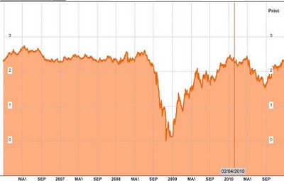
What about the argument that an inflation rate below the Fed’s target is alone enough to rationalize the unorthodox QE2 policy? I do not agree with this because the current low interest rate policy without QE2 is what is appropriate to deal with inflation being below the target. For example, the Taylor rule says that the federal funds rate is where it is because inflation is below its target. In other words that low interest rate policy means that monetary policy is doing what it should be doing to combat “too low” inflation, without QE2. Moreover, I think it would have been much harder to drum up support for QE2 based solely on deflationary concerns. As the Bloomberg graph below on breakeven inflation (USGGBE10) shows, the dip in expected inflation was quite small in 2010 and an argument based on that alone would not have carried the day in my view.

I have long been in favor of the Fed setting a target for inflation but not for unemployment. Here is a paper I gave at the 1996 Jackson Hole conference which explains why. In brief, by trying to focus on unemployment the Fed has actually increased unemployment. That was true in the 1970s and it is true recently: If the Fed had not kept interest rates so low when inflation was rising and the economy was growing in the 2002-2005 period, then we would have avoided much of the boom and the bust which eventually caused the devastating increase in unemployment.

One source of disagreement in debates about the mandate (which I tried to clarify in the 1996 paper) is confusion over the difference between the Fed’s goals and what the Fed reacts to. These are two different things. In particular, Sumerlin’s assessment that the Fed should react to credit aggregates is not inconsistent with the proposed changes in the mandate. Just as cutting interest rates in a recession when GDP falls below potential is an essential part of achieving a price stability goal in the framework of economic stability, so may be raising interest rates in a credit boom. The key idea is for the Fed to have and to lay out a strategy to achieve its goal. The strategy could entail credit aggregates, but that is a debate about how to achieve the mandate, not about the mandate itself.
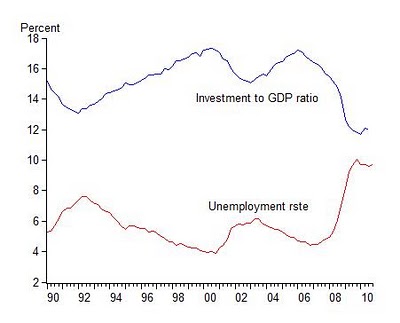
Posted in Monetary Policy | Comments Off on Impacts of Proposed Changes in the Fed’s Mandate

Putting New Fed Policy in the Economics Textbooks

Every Friday the economists at JP Morgan issue a useful compendium of facts and analysis called Global Data Watch. I’ve been reading GDW for many years, and I recall the days when it was only available in the paper edition.

Last Friday the economists moved a bit outside their data lane into undergraduate teaching with a major criticism that economics textbooks failed to teach students about the increase in excess reserves in the past two years. Their piece is called Blame the Textbook, Not the TA, for the Money Multiplier Confusion. Of course textbooks are not updated every week like GDW so it takes a while for them to reflect the latest developments. Nevertheless, the latest edition of my Principles of Economics text with Akila Weerapana, which has already been out for a year and a half now, does cover this increase in reserves and related developments. On page 635 of the 6th Edition, the Global Financial Crisis Edition, there is an explanation for the massive increase in excess reserves in a section called “The Explosion of Reserves and the Reserve Ratio in 2008.” I agree that it is important to teach students these developments in monetary economics and policy, so I reprint that section below. By the way there is an explanation of quantitative easing on page 750 of the same text.

From Principles of Economics, p. 635

“Banks sometime hold more than the required amount of reserves at the Fed and the reserve ratio can rise above the required reserve ratio. In our examples so far we have assumed that the reserve ratio is constant. In this section we explain what can happen when the reserve ratio changes. We focus on a particularly interesting real world example.
“In the fall of 2008 reserves at the Fed started increasing at a very rapid rate. As in our examples in the previous section, the Fed increased reserves by purchasing bonds and paying for them by creating deposits. However, in this case the Fed purchased very large amounts of bonds and other securities issued by private firms rather than the Federal government as it usually does. And it also made loans to private financial firms in an effort to contain the financial crisis. The Fed reasoned that by buying the bonds it could drive the interest rate on those bonds down which would ease the financial crisis. It also reasoned that making loans to certain financial firms would help them avoid bankruptcy and reduce risks to the financial system.
“When the Fed purchased these bonds and made the loans it paid for them by creating reserves—crediting banks with deposits at the Fed. The increase in reserves was unprecedented. Figure 4 shows how large, sudden, and unusual the increase was. After remaining relatively steady, reserves exploded in the fall of 2008. They increased from $44 billion in August 2008 to $858 billion in January 2009, more than a 20 fold increase.
Demand deposits at banks also increased as a result of this increase in reserves, which is not surprising given the connection between deposits and reserves explained in the previous section. The increase in demand deposits at banks is also shown in Figure 4. 
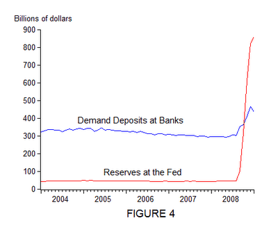
“Note that the increase in demand deposits was not as large as one would expect if the reserve ratio was constant. In fact, as shown in Figure 5, the reserve ratio was not constant. It was nearly constant for a number of years but then increased sharply in the fall of 2008 as banks chose to hold some of the large increase in reserves as excess reserves over the amount they were required to hold. In other words they decided not to lend out all the reserves. Banks did not lend out all the reserves because there was not enough demand for loans and because they were concerned about risks.
“The increase in demand deposits in turn increased the money supply because demand deposits are part of the money supply. Recalling earlier periods of high money growth, some people became concerned that the increase in the money supply would cause inflation, and they criticized the Fed for increasing the money supply by such a large amount. However, the Fed indicated that it did not see inflation as a problem. Policy officials were more concerned about the financial crisis. They indicated that if inflation picked up they would be able to reduce the amount of reserves and reduce deposits and the money supply.”
Posted in Teaching Economics | Comments Off on Putting New Fed Policy in the Economics Textbooks

Futures Market Forecast of a Federal Funds Rate Increase Likely to be Appropriate

According to the federal funds futures market, the Fed will begin raising rates sometime next year—with the federal funds rate reaching about ½ percent by December 2011. In fact, rising rates next year has been the implicit forecast of the futures market for the past year—except for the month of October during which many FOMC members were promoting quantitative easing. As this chart of the price of a December 2011 futures contract shows, a year ago the forecast was for a funds rate of over 2 percent next by the end of 2011. (The implicit forecast is obtained by subtracting the price in the chart from 100). Expectations of tightening have been rising again since the start of November, though thus far by a small amount.

This forecast is consistent with the Taylor rule and most recent forecasts for GDP growth and inflation. In fact, in my view it understates the interest rate that is likely to be appropriate by next December.

Most recent data (through the 3rd quarter) show that the inflation rate is about 1.2 percent (GDP deflator over the last four quarters) and the GDP gap is about 4.8 percent (average of San Francisco Fed survey). This implies an interest rate of 1.5 X1.2 + .5X(-4.8) + 1 = 1.8+ -2.4 +1 = .4 percent which is close to where we are now. But most likely GDP growth will turn out to be above potential growth in the 4th quarter bringing the gap down (Macro Advisers are projecting 3 percent with potential at 2.25 percent and JP Morgan is projecting 3.5 percent). Inflation is also very like to rise by this measure. For these reasons an increase in the federal funds rate next year is consistent with the Taylor rule.

Posted in Monetary Policy | Comments Off on Futures Market Forecast of a Federal Funds Rate Increase Likely to be Appropriate

Stimulus Math: Many Multiples of Nothing is Still Nothing

In an article in tomorrow’s Wall Street Journal, John Cogan and I review our research showing why the 2009 stimulus package did little to stimulate the economy, despite its large size. The reserch continues our earlier work showing why the temporary increases in transfers and tax rebates in the 2008 and 2009 stimulus packages did not work to stimulate the economy. Tomorrow’s article reports data showing that state and local governments did not increase their purchases of goods and services—including infrastructure—even though they received large grants in aid from the federal government. Instead they used the grants largely to reduce the amount of their borrowing as the following graph dramatically shows. 
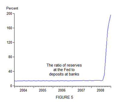
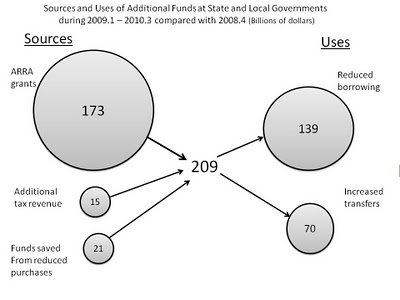
As American Recovery and Reconstruction Act (ARRA) grants from the federal government rose, the amount of net borrowing by state and local governments declined. The data come from the Bureau of Economic Analysis, Department of Commerce. The level of purchases is much less than government officials predicted when ARRA was passed in early 2009.

Posted in Stimulus Impact | Comments Off on Stimulus Math: Many Multiples of Nothing is Still Nothing