The Fed’s announcements yesterday increase monetary policy uncertainty in two fundamental ways.

Quantitative Easing on Steroids?

First, the new quantitative easing announcement implies a gigantic increase in the size of the Fed’s balance sheet and thus effectively an amplification of the policy risks and uncertainty which I have discussed, for example, in this oped with George Shultz and other colleagues in September. The Fed now plans to purchase $85 billion a month of longer-term Treasury and mortgage backed securities until there is substantial improvement in the labor market, which requires a completely unprecedented increase in reserve balances as illustrated in this chart.

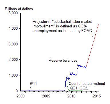
The chart shows reserve balances held by banks at the Fed. These are used to finance the large scale asset purchases.  The chart assumes that substantial labor market improvement is defined by the 6.5% unemployment rate the Fed is using to assess when to raise interest rates. Thus, assuming the central tendency forecast of the FOMC, the announced buying spree will bring reserve balances to about $4 trillion in mid-2015. The risk is two-sided. If the Fed does not draw down reserves fast enough during a future exit, then it will cause inflation. If it draws them down too fast, then it will cause another recession.

Another Great Deviation On the Way?

Second, the new state-based zero interest rate policy will lead to interest rates far below levels that created good performance in the past and close to levels that eventually created high unemployment. In an effort to explain the new policy during the press conference yesterday, Ben Bernanke referred to the Taylor rule, saying:

“So it’s really more like a reaction function or a Taylor rule if you will. I don’t want–I’m–I’ll get it–I’m ready to get the phone call from John Taylor. It is not a Taylor rule but it has the same feature that it relates policy to observables in the economy such as unemployment and inflation.”

In fact, the Fed’s new state-based policy calls for the federal funds rate to stay way below the Taylor rule, as did the calendar-based policy. You can see this deviation in two ways: a chart or some algebra.

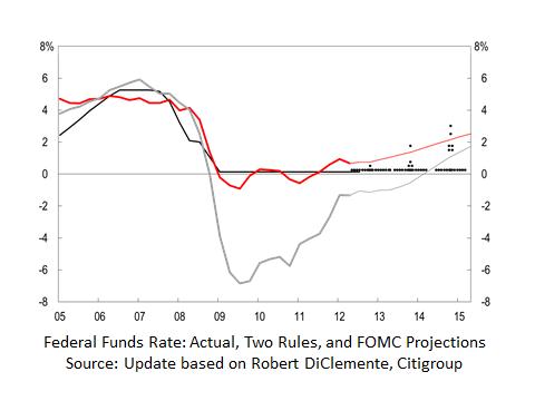
Consider the following chart (an updated version of a chart due to Bob DiClemente) which I used in my talk last month at the Cato Institute. The red line shows the interest rate according to the Taylor rule with the future values based on FOMC forecasts for inflation and growth. The zero interest rate forecasts by most FOMC members (shown by the dots) for mid-2015—a time when, they forecast, the unemployment rate will be about 6.5 percent—are more than 2 percentage points below the Taylor rule. (The gray line is a version of the Taylor rule used by Janet Yellen and others at the Fed.)

You can also plug in values into the Taylor rule:

R = 2 + π + 0.5(π – 2) + 0.5Y

where R is the federal funds rate, π is the inflation rate, and Y is the GDP gap.

Assume that Y = -2(U-5.5) where U is the unemployment rate and 5.5 is the long-term unemployment rate implied by FOMC projections. Then when the unemployment rate is 6.5% and the inflation rate is 2%, the interest rate is 2+2 -1 = 3%. So there is a 3 percent deviation.

The last time the deviation between the Taylor rule and the actual rate was this large was in the “too low for too long” period of 2003-2005 which helped create the boom which led to the bust, the financial crisis, and the recession. High unemployment was the result. The deviation was also this large during the economic mess of the 1970s. High unemployment, along with high inflation, was the result then too.

Comparison with Larry Ball’s Calculations

Larry Ball did a very similar algebraic calculation with similar conclusions about the difference between the Fed’s future policy rate and the Taylor rule, which Greg Mankiw posted on his blog earlier today.

However, Larry finds that the actual interest rate was not below the Taylor rule in the 2003 period. This result is contrary to empirical research by George Kahn, me and others. The difference may be due to Larry’s using an implied coefficient on the output gap which is larger than .5. Nevertheless, the deviation Larry uncovers is much larger than in the 1970s, which in itself raises risks.